Scientific visualization of transport and diffusion

Open computational physics project

Radioactive Pollution Transport in Flowing Water

An interactive presentation of the convection–diffusion model and MATLAB simulations for instantaneous radioactive releases in one, two, and three dimensions.

Explore simulations View source

Project overview

From pulsed neutron activation to transport modeling

In an earlier study, we showed how Pulsed Neutron Activation (PNA) analysis could be implemented to estimate the flow speed in a one-dimensional pipeline [1]. The neutron capture by target stable nuclides, like Oxygen-16 in water, leads to radioactive Nitrogen-16 emitting high-energy gamma-rays, which travels with flowing water in a channel and can be detected and analyzed downstream in the pipe to get information about its average transport time. Then by having the traveled distance, i.e., the distance between the gamma source and the gamma detector, one can obtain the speed of the activity and, consequently, the flow speed and mass rate in the pipeline. This report shows how we can extend the technique to study pollution diffusion, including radioactive pollution, in a three-dimensional stream.

[1]

M. R. Hadizadeh, An Overview of the Application of Pulsed Neutron Activation in Flow Measurements, Nuclear Technology (2019), 1–9.

Mathematical model

Transport equation in three dimensions

The transport of pollution in a three-dimensional stream with the diffusion coefficient $D$ flowing with velocity v, when there is source or sink ${\cal R}$ , can be described by the convection-diffusion equation

\frac{\partial C}{\partial t}=\nabla\cdot(D\,\nabla C)-\nabla\cdot(C\,\textbf{%v})+{\cal R},

(1)

where $C$ is the pollution concentration. The transport equation (1) in a Cartesian coordinate system, where the fluid is moving with the constant velocity of v can be represented as

$\displaystyle\frac{\partial C(x,y,z,t)}{\partial t}$	$\displaystyle=$	$\displaystyle\left(D_{x}\frac{\partial^{2}C(x,y,z,t)}{\partial x^{2}}+D_{y}%\frac{\partial^{2}C(x,y,z,t)}{\partial y^{2}}+D_{z}\frac{\partial^{2}C(x,y,z,t%)}{\partial z^{2}}\right)$	(2)
	$\displaystyle-$	$\displaystyle\left(v_{x}\frac{\partial C(x,y,z,t)}{\partial x}+v_{y}\frac{%\partial C(x,y,z,t)}{\partial y}+v_{z}\frac{\partial C(x,y,z,t)}{\partial z}\right)$	(3)
	$\displaystyle+$	$\displaystyle{\cal R}(x,y,z,t)$	(4)

where

•
$C(x,y,z,t)$ : the pollution concentration at location $(x,y,z)$ and time $t$ ,
•
$D_{x},\ D_{y},\ D_{z}$ : the horizontal and vertical components of diffusion coefficient. For an anisotropic medium, like rivers and lakes, $D_{x},\ D_{y},D_{z}$ are unequal, while for an isotropic medium, the diffusion proceeds at the same rate in horizontal and vertical directions,
•
$v_{x},\ v_{y},\ v_{z}$ : the flow velocity components in the $x$ , $y$ , and $z$ directions. They are constant in each spatial direction for the studied contaminated region,
•
${\cal R}(x,y,z,t)$ : the pollution emission at location $(x,y,z)$ and time $t$ .

Considering the boundary conditions, the pollution concentration must converge to zero as $x$ , $y$ , or $z$ tends to infinity

	$\displaystyle\lim_{x\to\pm\infty}C(x,y,z,t)\rightarrow 0,$		(5)
	$\displaystyle\lim_{y\to\pm\infty}C(x,y,z,t)\rightarrow 0,$		(6)
	$\displaystyle\lim_{z\to\pm\infty}C(x,y,z,t)\rightarrow 0;$		(7)

and the initial condition,

\displaystyle C(x,y,z,t=0)=M\ \delta(x-x_{0})\ \delta(y-y_{0})\ \delta(z-z_{0}),

(8)

where $M$ is the released point-source pollution at location $(x_{0},y_{0},z_{0})$ and time $t=0$ . In a 1D model in $x-$ direction, $M\equiv\frac{M}{L_{y}\cdot L_{z}}$ represents the surface mass flux or total mass per unit area, where $L_{y}\cdot L_{z}$ is the area scale of neglected dimensions. Similarly, in a 2D model in the $x-y$ direction, $M\equiv\frac{M}{L_{z}}$ represents linear mass flux or total mass per unit length, where $L_{z}$ is the area scale of neglected dimension. The total mass of pollution at time $t$ must be equal to the number of undecayed pollution at time $t$ , i.e. $M(t)$ . So, the boundary and initial conditions are

\int_{{v}d{v}}\,C(x,y,z,t)=M(t).

(9)

If the source of the contamination is radioactive material, the mass of undecayed material at time $t$ is given by the radioactive decay law

M(t)=M_{0}\,e^{-\lambda\,t},

(10)

where $\lambda=\frac{\ln(2)}{T_{1/2}}$ is the decay constant for the induced radioactive material. For an instantaneous point-source pollution

	$\displaystyle C(x,y,z,t)$	$\displaystyle=$	$\displaystyle\frac{M_{0}}{(4\pi t)^{3/2}(D_{x}D_{y}D_{z})^{1/2}}$		(11)
		$\displaystyle\times$	$\displaystyle\exp{\left(-\frac{(x-x_{0}-v_{x}t)^{2}}{4D_{x}t}-\frac{(y-y_{0}-v%_{y}t)^{2}}{4D_{y}t}-\frac{(z-z_{0}-v_{z}t)^{2}}{4D_{z}t}-\frac{\ln(2)}{T_{1/2%}}\,t\right)}.$		(12)

Computational toolkit

Numerical results

To study the pollution diffusion from a radioactive source in a river or lake, we develop a computational toolkit in Matlab to solve the transport equation and calculate pollution concentration as a function of time at different locations.

Instantaneous release in a one-dimensional stream

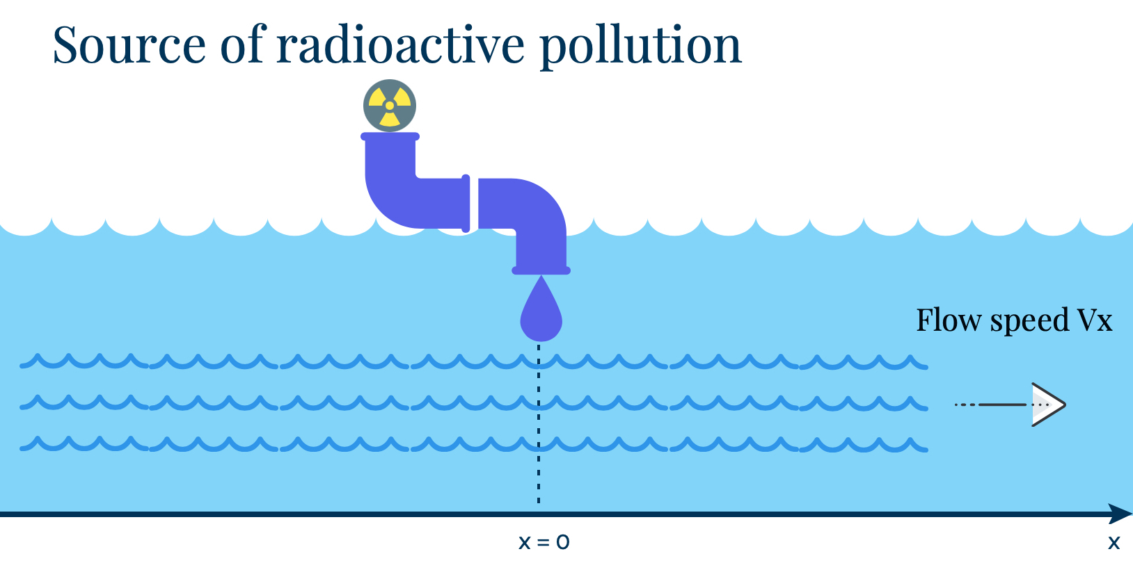
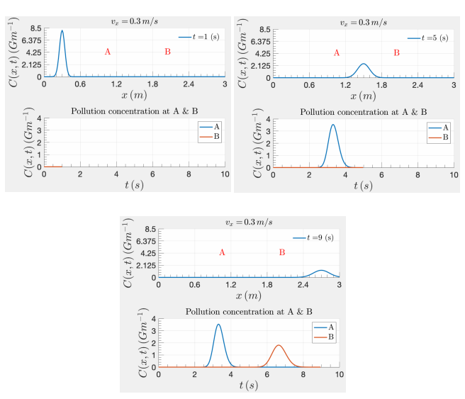
For the first implementation, we study the diffusion of radioactive pollution from an instantaneous release in a 1D water canal flowing at a constant speed. In the image above, we show the pollution release in a one-dimensional water canal flowing in the x direction with a constant speed v_x. The Matlab scripts listed in Appendix A, create 2D motion plots (in AVI and GIF formats) for the evolution of pollution concentration.

Time evolution of one-dimensional pollution concentration

FIG. 2: Few screenshots of 2D motion plots obtained from the Matlab toolkit that calculates the pollution diffusion obtained from instantaneous release from radioactive neutron source 16N (with a half-life T_1/2 = 7.13 s) as a function of time t and distance x, in a water canal flowing with a constant speed v_x = 0.3 m/s and a diffusion coefficient

Animated one-dimensional pollution transport simulation

Open 1D MATLAB files

Instantaneous release in a two-dimensional stream

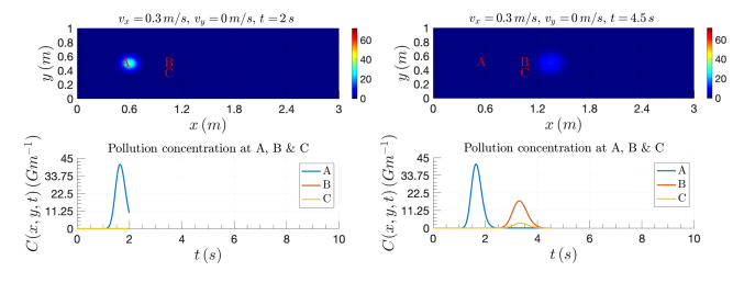
In this section, we study the diffusion of radioactive pollution from an instantaneous release in a 2D water stream flowing at constant speeds v_x and v_y in the x and y directions. The Matlab scripts listed in Appendix B, create 2D motion plots (in AVI and GIF formats) for the evolution of pollution concentration from a release at point ( x₀, y₀).

Snapshots of two-dimensional pollution concentration

FIG. 3: Few screenshots of 2D motion plots obtained from the Matlab toolkit that calculates the pollution diffusion obtained from instantaneous release from radioactive neutron source 16N (with a half-life T_1/2 = 7.13 s) at (x₀ = 0 m, y₀ = 0.5 m) as a function of time t and distances x and y, in a water river flowing with a constant speeds v_x = 0.3 m/s and v_y = 0.0 m/s and diffusion coefficients D_x = D_y = 0.001.

Animated two-dimensional pollution transport simulation

Open 2D MATLAB files

Instantaneous release in a three-dimensional stream

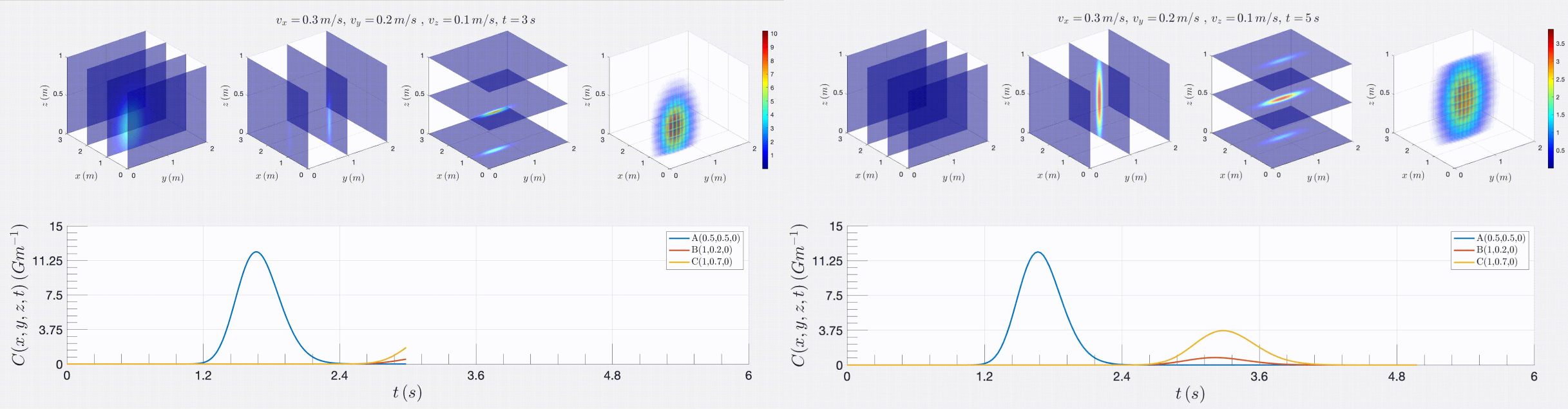
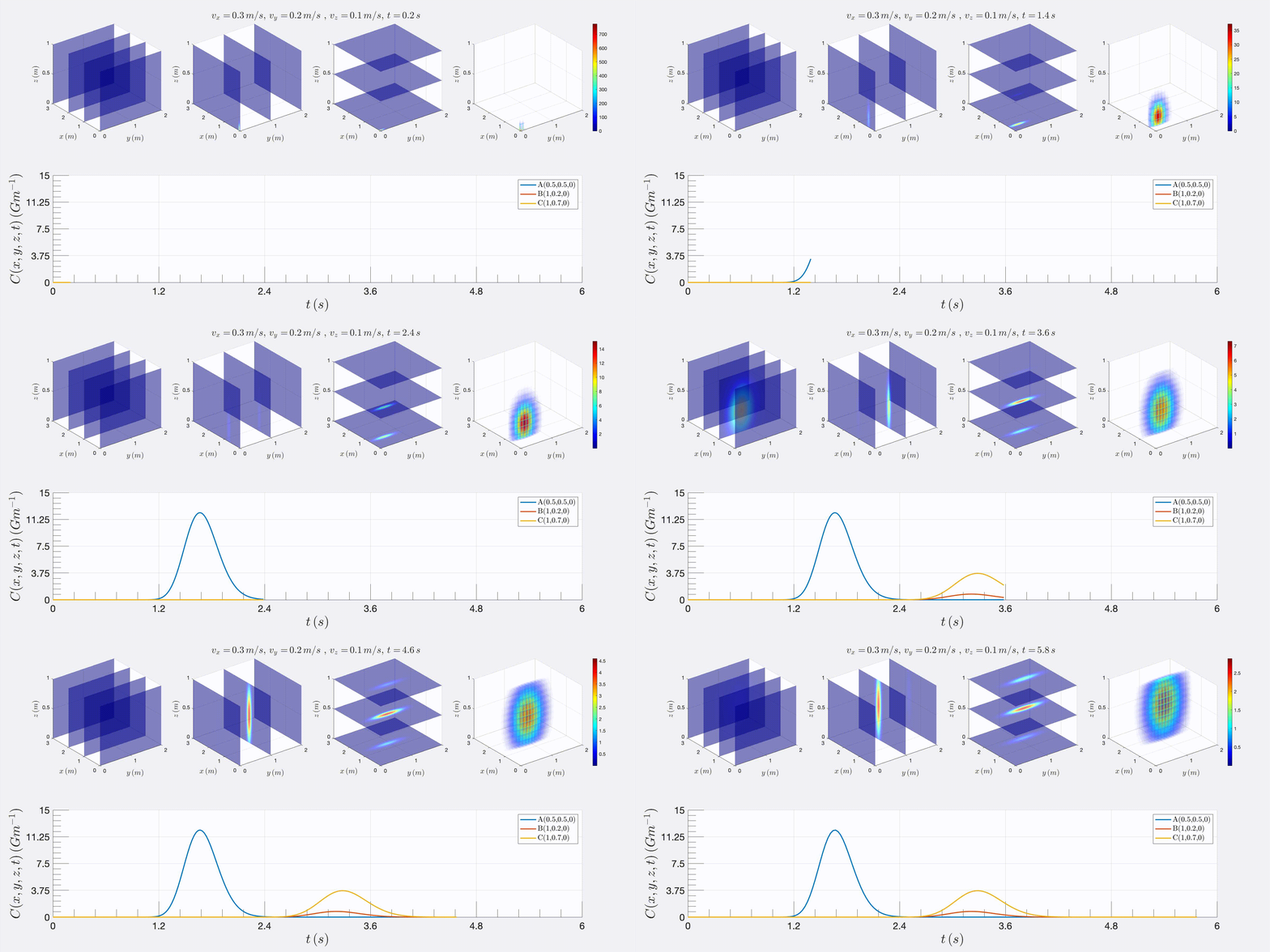
In this section, we study the diffusion of radioactive pollution from an instantaneous release in a 3D water stream flowing at constant speeds v_x, v_y, and v_z in the x, y, and z directions. The Matlab scripts listed in Appendix B, create 3D motion plots (in AVI and GIF formats) for the evolution of pollution concentration from a release at point (x₀, y₀, z₀).

Snapshots of three-dimensional pollution concentration

FIG. 3: Few screenshots of 3D motion plots obtained from the Matlab toolkit that calculates the pollution diffusion obtained from instantaneous release from radioactive neutron source 16N (with a half-life T_1/2 = 7.13 s) at (x₀, y₀, z₀) as a function of time t and distances x and y, in a water river flowing with a constant speeds v_x = 0.3 m/s, v_y = 0.2 m/s, and v_z = 0.1 m/s and diffusion coefficients D_x = 0.001 D_y = D_z = 0.01.

Animated three-dimensional pollution transport simulation

Open 3D MATLAB files

Contact

Interested in educational or research collaboration?

I welcome inquiries about educational and research collaborations of any kind, including joint projects, computational methods, classroom applications, and opportunities to extend these open resources.

Dr. Mohammadreza Hadizadeh

Professor of Physics

College of Engineering, Science, Technology and Agriculture
Central State University

O: 937 376-6273
E: mhadizadeh@centralstate.edu
W: https://people.ohio.edu/hadizadm/