
Open-source Interactive Website for Exciton modeling via the lippmann-schwinger equation
Solve 2d quantum bound states in your browser
This website provides an open, browser-based platform for solving the Lippmann–Schwinger (LS) equation in two dimensions. It delivers executable Jupyter notebooks that take users from parameter setup and Gauss–Legendre discretization to numerical solution, binding-energy evaluation, Hamiltonian-expectation checks, and wave-function visualization. Ready-to-run case studies—2D hydrogenic (Coulomb), deuteron (Malfliet–Tjon), and exciton (Rytova–Keldysh)—link compact theory to reproducible momentum-space computations. Hosted on GitHub Pages, it is free, zero-install, and open for community contributions.
Lippmann–Schwinger Equation for 2B Bound States in 2D
The starting point for a 2B bound state with reduced mass \(\mu\) is the time-independent Schrödinger equation \[(H_0 + V)\,|\Psi\rangle = E\,|\Psi\rangle\]where\(H_0\) is the free Hamiltonian, \(V\)is the interaction, \(E<0\) is the binding energy, and \(|\Psi\rangle\)is the corresponding bound state wave function. Rearranging the equation above gives the homogeneous LS equation for a bound state\[|\Psi\rangle = G_0(E)\,V\,|\Psi\rangle, \qquad G_0(E) \equiv \frac{1}{E - H_0}\] which expresses the state in terms of \(G_0(E)\)and the interaction. In a momentum basis\(|\mathbf p\rangle\), adopting the completeness the free propagator\(\int \! d^2 p\, |\mathbf p\rangle\langle \mathbf p| = 1\), the LS equation projects to\[\psi(\mathbf p) = \frac1E - \dfrac{p ^ 2}{2\mu}\, \int_0^\infty \! dp'\, p' \int_0^2\pi \! d\phi'\, V(\mathbf p,\mathbf p')\, \psi(\mathbf p')\]where \(\psi(\mathbf p) \equiv \langle \mathbf p| \Psi\rangle\) and\(V(\mathbf p,\mathbf p') \equiv \langle \mathbf p| V | \mathbf p' \rangle\). For central interactions in 2D, it is convenient to separate the angular dependence by a partial-wave (PW) expansion, which reduces LS equation to a one-dimensional integral equation for each angular-momentum channel \(m\)\[\psi_m(p) = \frac1{E - \dfrac{p ^ 2}{2\mu}} \int_0^\infty \! dp'\, p'\, V_m(p,p')\, \psi_m(p').\]The PW-projected kernel can be obtained from the angular integration in momentum space, \[\begin{aligned}V_m(p, p') = \int_0^{2\pi} d\phi' \, V(p, p', \phi') \cos(m \phi') \equiv \int_0^\infty dr r \, J_m(pr) V(r) J_m(p'r).\end{aligned}\]with \(J_m\) the Bessel function of the first kind. The PW representation for each \(m\) reduces the 2D integral equation to a one-dimensional radial form. This framework is used throughout to compute 2D bound states, e.g., hydrogenic systems with Coulomb interactions and the deuteron with Yukawa-type interactions, and, in particular, excitons with the RK interaction, within a momentum-space LS scheme.
A convenient internal consistency check for a numerically obtained 2B binding energy and wave function is to compare the eigenvalue \(E\) from the LS equation with the Hamiltonian expectation value, \(\langle H \rangle = \langle H_0 \rangle + \langle V \rangle\), evaluated using the corresponding momentum-space wave function. The degree of agreement between \(E\) and \(\langle H \rangle\) provides a direct measure of the numerical accuracy of the method. For a given PW channel\(m\), with the wave function normalization \[\int \! d^2p\, \psi^2(\mathbf p) = 2\pi \int_0^\infty \! dp\, p\, \psi_m^2(p) = 1.\] The Hamiltonian expectation value, expressed in terms of the kinetic and potential contributions, reads\[\begin{aligned}\langle H \rangle &= \langle H_0 \rangle + \langle V \rangle, \\[3pt] \langle H_0 \rangle &= 2\pi \int_0^\infty \! dp\, p\;\frac{p ^ 2}{2\mu}\, |\psi_m(p)|^2, \\[3pt] \langle V \rangle &= 2\pi \int_0^\infty \! dp\, p \int_0^\infty \! dp'\, p'\; \psi_m(p)\, V_m(p,p')\, \psi_m(p') \,.\end{aligned}\]
Numerical Implementation
To numerically solve the LS integral equation for a 2B bound state in 2D, represented in the PW framework, the integral equation should be transformed into a discretized form that can be solved iteratively or through matrix diagonalization. To efficiently handle the integrals, variable transformations are introduced to map the infinite domains of momentum \(p\), spatial coordinate \(r\), and angle\(\phi\) onto finite intervals. The transformations are defined as: \[p,p', r = \frac{1 + x}{1 - x}, \quad \phi' = \pi (1+x), \quad x \in [-1,1],\]where \(x\) is a variable spanning the interval \([-1, 1]\), suitable for integration using Gaussian-Legendre quadrature. The discretized form of the integral equation for the wave function \(\psi_m\) becomes an eigenvalue problem:\[\lambda \ \psi_m = {\cal K}(E) \, \psi_m,\] where \({\cal K}(E)\)represents the integral kernel operator dependent on the binding energy \(E\). The eigenvalue \(\lambda\) is used as a criterion to verify the solution. The binding energy \(E\) is determined by solving for the eigenvalue \(\lambda = 1\). This involves iteratively searching over initial guesses for \(E\)until convergence is achieved. A tolerance of \(10^-6\) is set for the eigenvalue condition, ensuring high accuracy in the computed energy.
The iterative search procedure can be outlined as follows:
Select two initial guesses for the binding energy E.
Construct the kernel \({\cal K}(E)\) for each chosen energy.
Solve the eigenvalue problem \(\lambda \, \psi_m = {\cal K}(E) \, \psi_m\) to obtain \(\lambda\) and the corresponding wave function \(\psi_m\) for both initial guesses.
Using these two initial pairs \((E, \lambda)\), perform a linear fit to predict the next energy value for which \(\lambda = 1\).
Iterate the process with the updated energy values until \(\lambda\) converges to \(1\) within the specified tolerance.
The kernel \({\cal K}(E)\) is diagonalized at each step, which allows for the extraction of both the eigenvalue \(\lambda\) and the wave function \(\psi_m\). Efficient numerical techniques such as matrix diagonalization, implemented through libraries like LAPACK, or iterative solvers like the Lanczos algorithm, can be employed for this purpose.
Systems Studied
To ensure the robustness and accuracy of our computational framework, a critical first step is validating the numerical methods against established benchmarks. For this purpose, we compare our simulated results for the 2D hydrogenic atom and the 2D deuteron system with well-known theoretical findings. These systems serve as ideal case studies: the hydrogenic atom, with its fundamental Coulomb potential, provides an exact analytical benchmark for bound states, while the deuteron, modeled with the more intricate MT potential, demonstrates the framework’s ability to handle complex nuclear interactions. By showing strong agreement between our computational outputs and trusted reference values, we establish confidence in the accuracy and reliability of our algorithms. This rigorous validation provides the essential foundation for applying our methods to more complex systems, such as excitons in 2D materials, where the RK potential is used to probe the influence of screening length and dielectric constants on binding energies and wavefunctions
Hydrogenic atom in 2D
We begin with the 2D hydrogenic system, a well-established case that provides an ideal benchmark for testing the accuracy of our numerical method. In contrast to its three-dimensional analogue, the 2D system exhibits distinctive features in its energy spectrum and wave function behavior arising from the reduced dimensionality. In this section, we present both analytical and numerical treatments of the problem, working in natural units where \(\hbar c = e = m = 1\). The 2B potential energy between a nucleus of charge \(Z\) and a single electron in configuration space is given by \[V(r) =-\dfrac{Z}{r},\] which can be expressed in momentum space as\[V({\mathbf p}, \mathbf p') =\dfrac{-Z}{2\pi \vert {\mathbf q}\vert}, \quad \mathbf q= \mathbf p-{\mathbf p}'.\]The analytical solutions of the LS integral equation for the 2B binding energy levels are given in Ref. \[E_{exact} = -\dfrac{Z ^ 2 m}{4\left(n + 1/2\right)^2}, \quad n = 0, 1, 2, \ldots\] The exact energy levels for 2D hydrogenic atoms offer a clear reference for comparison. Evaluating the agreement between our computed values and the known analytical results allows us to assess the reliability of the approach and identify potential issues at an early stage. Establishing this validation is essential before extending the method to more complex systems, such as excitons or deuterons. The results of this comparison are presented in Table 1, showing that our numerical values closely match the exact energy levels of the 2D hydrogenic atom. The relative errors are very small, less than 0.4% for the ground state and the first three excited states, demonstrating the accuracy and reliability of our method.
Table 1 Comparison of analytical (\(E_{num}\)) and numerical (\(E_{num}\)) 2B binding energies, obtained from Eqs. (14) and (4), respectively, for the 2D hydrogenic atom with partial wave \(m=0\) and nuclear charge \(Z=2\). Calculations employ \(500\) grid points for the magnitude of the relative momentum and \(40\) points for the angular variables.
| n | \(E_exact\) | \(E_{Num}\) | \(\left(\dfrac{E_{exact} - E_{num}}{E_{exact}}\right) \times 100 \%\) | |||
|---|---|---|---|---|---|---|
| 0 | -4.00000 | -3.99928 | 0.01800 | |||
| 1 | -0.44444 | -0.44441 | 0.00700 | |||
| 2 | -0.16000 | -0.16017 | 0.10625 | |||
| 3 | -0.08163 | -0.08193 | 0.36751 |
Fig. 1 complements the binding‐energy results in Table 1 by showing momentum-space hydrogenic wave functions for \(n=0-3\). The plots depict \(\psi^{(n)}_{m}(p)\) versus relative momentum \(p\), highlighting how the momentum distribution varies with the energy level. The ground state exhibits a broader high-\(p\)distribution, whereas excited states (\(n=1,2,3\)) develop nodes and shift weight toward lower \(p\), consistent with their larger spatial extent in configuration space.
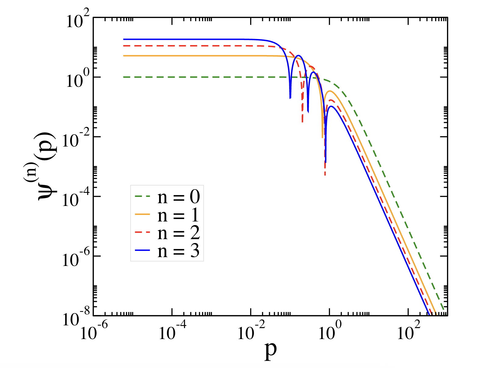
Figure 1 Ground (\(n=0\)) and first three excited (\(n=1-3\)) momentum-space wave functions \(\psi^{(n)}_{m}(p)\) of the 2D hydrogenic atom for partial wave \(m=0\) and nuclear charge \(Z=2\) as functions of relative momentum\(p\). States correspond to the numerical binding energies in Table 1
Deuteron in 2D
This section presents the numerical simulation of the deuteron, the bound state of one proton and one neutron, in 2D using the MT potential, written as a sum of repulsive and attractive Yukawa terms, \[V(r) = V_r \frac{e ^ {-\mu_r r}}{r} + V_a\frac{e ^ {-\mu_a r}}{r},\] where \(V_r\) and \(V_a\) are the strengths of the repulsive and attractive components, respectively, and \(\mu_r\) and \(\mu_a\) are the corresponding range parameters. The potential transforms to momentum space as \[V(\mathbf p, \mathbf p') = \frac{1}{2\pi}\left( \frac{V_r}{\sqrt{q ^ 2 + \mu_r^2}} + \frac{V_a}{\sqrt{q ^ 2 + \mu_a^2}} \right), \quad q = | \mathbf p- \mathbf p' |.\]The parameter sets for the two MT models used in our calculations are listed in Table and the corresponding momentum-space potentials \(V(q)\) are plotted in Fig. as functions of the momentum transfer \(q\).
Table 2 Parameter sets for the two MT potential models used in our calculations.
| MT-model | \(V_a \, \text{(MeV fm)}\) | \(\mu_a \, (\text{fm}^{-1})\) | \(V_r \, \text{(MeV fm)}\) | \(\mu_r \, (\text{fm}^{-1})\) |
|---|---|---|---|---|
| Model-1 | \(-600.00\) | \(1.550\) | \(1438.7228\) | \(3.21\) |
| Model-2 | \(-600.00\) | \(1.550\) | \(0\) | \(0\) |
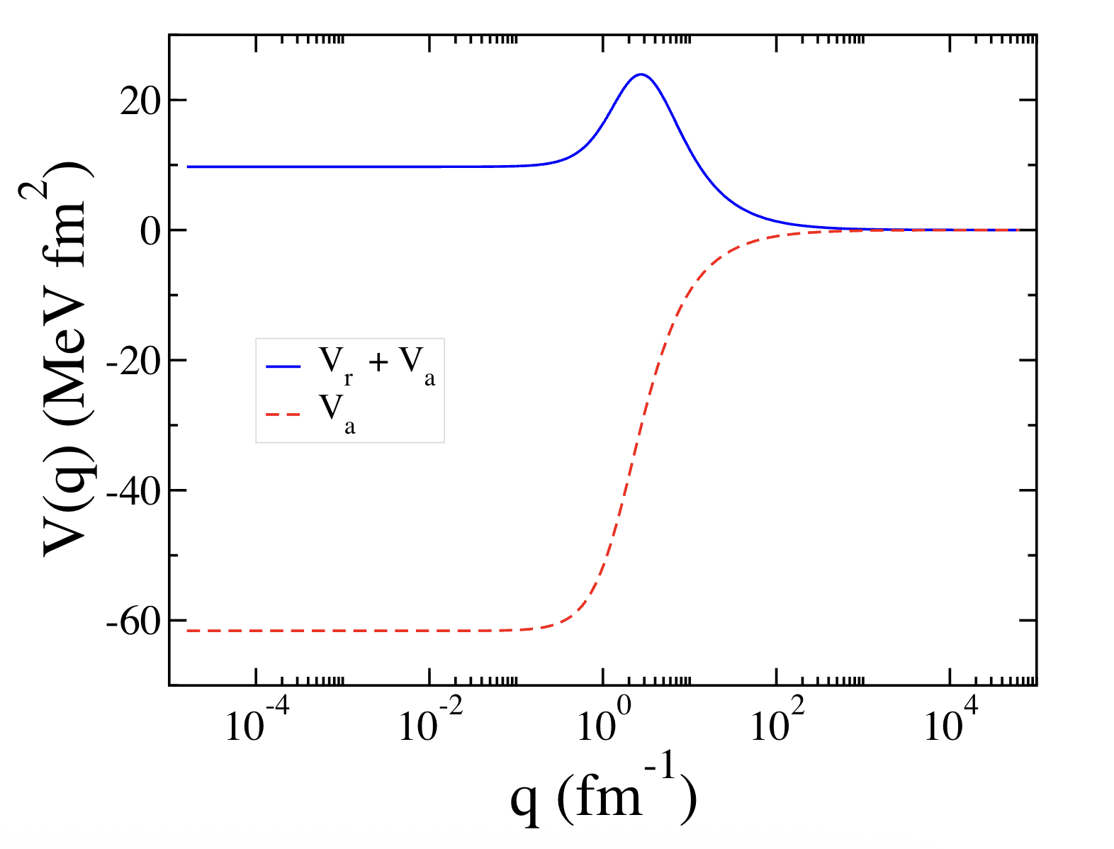
Figure 2 Comparison of the two MT potentials as functions of the momentum transfer \(q\).
In our calculations, we use the nucleon mass with \(\hbar^2/m = 41.47\ MeV \text·fm^2\). As shown in Table , the computed binding energies for the 2D deuteron differ markedly between the two MT models. This is expected: Model 1, which superposes repulsive and attractive Yukawa terms, supports only a single (ground) bound state, whereas Model 2, which is purely attractive, supports two deeper bound states (ground and first excited). The corresponding momentum-space wave functions are shown in Fig.The left panel (Model 1) displays a single ground-state wave function, \(\psi(p)\), versus relative momentum \(p\). The right panel (Model 2) presents two ground and excited bound states, labeled \(n=0\) and \(n=1\).
Table 3 Calculated 2D deuteron binding energies for the two MT potential models, using \(200\) grid points for the 2B relative-momentum magnitude and \(101\) grid points for the angular variables.
| \(E_{d}\) (MeV) | \(E^{(0)}_{d}\) (MeV) | \(E^{(1)}_{d}\) (MeV) | ||
|---|---|---|---|---|
| Model-1 | Model-2 | |||
| \(-6.246\) | \(-7806\) | \(-312.4\) | ||
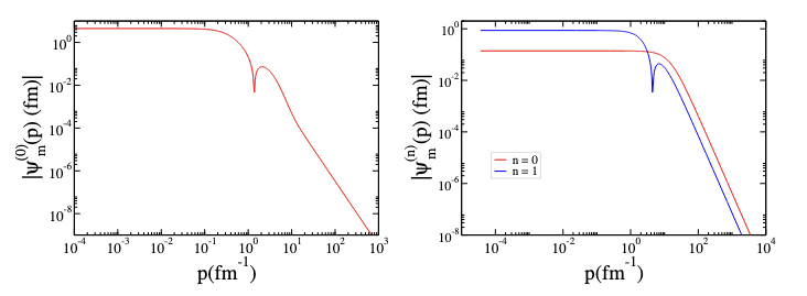
Figure 3 2D momentum-space deuteron wave functions \(\psi(p)\), computed with the MT potential: Model 1 (left) and Model 2 (right), plotted versus relative momentum\(p\).
Excitons in 2D Materials
Having validated the framework on 2D hydrogenic atoms and the deuteron, we now apply it to excitons-bound electron-hole pairs formed by Coulomb attraction that play a central role in the optical response of 2D materials. In this section we solve the LS integral equation for excitons using the RK potential. This yields exciton binding energies and wave functions, providing insight needed to predict exciton behavior in practical devices and to inform the design of materials with targeted optical properties. The RK potential accounts for nonlocal, distance-dependent dielectric screening in 2D materials, and thus models electron-hole interactions more accurately than a bare Coulomb potential. The explicit forms of the RK potential in configuration and momentum space are\[\begin{aligned}V(r) &=& -\dfrac{\alpha \hbar c \pi}{2 r_0 \kappa}\left[H_0\left(\dfrac{r}{r_0}\right)-Y_0 \left(\dfrac{r}{r_0}\right)\right], \cr V(\mathbf p,\mathbf p') &=& - \dfrac{1}{4\pi^2}\left( \dfrac{1}{4\pi \epsilon_0 \kappa} \dfrac{2\pi e^2}{q(1 + r_0 q/\kappa )}\right), \quad q = | \mathbf p- \mathbf p' |\end{aligned}\]where \(H_0\)and \(Y_0\) denote, respectively, the order-zero Struve function and the Bessel function of the second kind. Here \(r\) denotes the electron-hole separation, \(r_0\) is the screening length, and \(\kappa=(\epsilon_1+\epsilon_2)/2\) is the average environmental dielectric constant. The factor \(\epsilon_0/e^2=\big(4\pi\,\alpha\,\hbar c\big)^-1\) converts between the fine-structure constant and energy units. We use \(\alpha^-1=137.035999084\), \(\hbar c=1973.269804\ \text{eV}\!\cdot\!\text{Å}\), and the electron rest mass \(m_0=0.510998950\ \text{MeV}\). The material-dependent RK parameters used in our calculations are summarized in Table 4.
Table 4 Electron-hole RK potential parameters for monolayer TMDs, electron and hole effective masses \(m_e\), \(m_h\) (in units of \(m_0\)) and screening length \(r_0\) (Å), for MoS\(_2\), MoSe\(_2\), WS\(_2\), and WSe\(_2\); values from density functional theory in Ref. .
| Substance | \(m_e \ (m_0)\) | \(m_h \ (m_0)\) | \(r_0\)(Å) | |||||||||||
|---|---|---|---|---|---|---|---|---|---|---|---|---|---|---|
| MoS\(_2\) | 0.47 | 0.54 | 44.6814 | |||||||||||
| MoSe\(_2\) | 0.55 | 0.59 | 53.1624 | |||||||||||
| WS\(_2\) | 0.32 | 0.35 | 40.1747 | |||||||||||
| WSe\(_2\) | 0.34 | 0.36 | 47.5701 |
Our exciton binding energies for monolayer MoS\(_2\), MoSe\(_2\), WS\(_2\), and WSe\(_2\), computed with the RK momentum-space potential using the parameters in Table 4 and obtained by solving the LS integral equation are reported in Table 5. As a numerical self-consistency check, we also compare each binding energy with the Hamiltonian expectation value \(\langle H\rangle=\langle H_0\rangle+\langle V\rangle\) evaluated from the corresponding wave function. In all four materials, the relative percentage differences are well below \(3 \cdot 10^-6\%\), indicating that the momentum/angle discretization, kernel construction, and diagonalization are converged and the solutions are numerically reliable.
Table 5 Exciton binding energies and Hamiltonian expectation values for monolayer TMDs. with the corresponding Hamiltonian expectation values, \(\langle H\rangle=\langle H_0\rangle+\langle V\rangle\), along with their relative percentage differences. Calculations use \(500\) grid points in the relative momentum magnitude \(p\)and \(40\) in the azimuthal angle.
| \(E_{2B}\) (meV) | \(\langle H_0 \rangle\) (meV) | \(\langle V\rangle\) (meV) | \(\langle H\rangle\) (meV) | \(\vert \frac{\langle H \rangle- E_{2B}}{E_{2B}} \vert \times 100 \%\) | |
|---|---|---|---|---|---|
| MoS\(_2\) | \(-529.821\) | \(135.816\) | \(-665.637\) | \(-529.821\) | \(5.73 \cdot 10^-7\) |
| MoSe\(_2\) | \(-480.553\) | \(116.507\) | \(-597.060\) | \(-480.553\) | \(1.40 \cdot 10^-7\) |
| WS\(_2\) | \(-512.597\) | \(144.819\) | \(-657.416\) | \(-512.597\) | \(2.45 \cdot 10^-6\) |
| WSe\(_2\) | \(-460.118\) | \(124.665\) | \(-584.783\) | \(-460.118\) | \(1.38 \cdot 10^-7\) |
In Table 6, we show the convergence of exciton binding energies for the TMDs as a function of the number of mesh points in the relative momentum magnitude \(N_p\), together with an extrapolation to\(1/N_p \to 0\) (last column). The extrapolated values are in excellent agreement with Refs. across all materials, with relative percentage differences below \(0.3\%\).
Table 6 Exciton binding energies (meV) for different numbers of mesh points.
| \(N_p\) | 500 | 600 | 700 | 800 | \(\to \infty\) | |||
|---|---|---|---|---|---|---|---|---|
| Mo\(\text{S}_2\) | \(-529.821\) | \(-527.901\) | \(-526.718\) | \(-525.955\) | \(-524.872\) | |||
| MoSe\(_2\) | \(-480.553\) | \(-478.640\) | \(-477.460\) | \(-476.700\) | \(-475.753\) | |||
| W\(\text{S}_2\) | \(-512.597\) | \(-510.759\) | \(-509.613\) | \(-508.866\) | \(-507.613\) | |||
| WSe\(_2\) | \(-460.118\) | \(-458.303\) | \(-457.170\) | \(-456.426\) | \(-454.772\) |
Extending Beyond the Case Studies: General 2B Bound States in 2D
After the three example case studies, Hydrogenic atom in 2D, Deuteron in 2D, and Excitons in 2D materials, the following code is meant to serve as a general interactive environment for studying any two-body bound state in 2D, as long as the interaction is specified in configuration space as a function of the relative distance r. The core idea is simple: you provide a potential V(r) in configuration space, and the code handles the transformation to momentum space, builds the Lippmann–Schwinger kernel, and computes the binding energy and corresponding wave function.
In practice, you have three options: use one of the two pre-defined potentials or define a new potential in the build_V_r function:
Use the pre-defined Coulomb-like potential
Appropriate for hydrogenic systems or excitons where a long-range attractive interaction is dominant. You select this by choosing the Coulomb option in the potential_type setting.Use the pre-defined Malfliet–Tjon (MT) potential
Suitable for nuclear-type systems like the deuteron, where the interaction has both short-range repulsive and intermediate-range attractive parts. You select this by choosing the MT option in potential_type. The standard MT parameters are already coded, but you can adjust them if you wish to explore variations.Define your own custom potential in configuration space
For any other two-body system, you can choose the “custom” option in potential_type and then modify the “custom” section of the potential-building function to implement your desired interaction. This is where you directly specify how the potential depends on the radial coordinate r. By editing just this part of the code, you can explore a wide variety of model interactions without changing the rest of the numerical machinery.
Regardless of which option you choose—Coulomb, Malfliet–Tjon, or a custom interaction—it is essential to ensure that the mass parameter in the get_mass function is defined consistently with your physical problem and units. The mass determines how the kinetic term is treated and therefore has a direct impact on the resulting binding energy. When you introduce a new potential or change the physical system you are modeling, remember to update the mass definition in the configuration section of the script so that it matches your chosen units and physical context.
User Guide: Accessing, Editing, and Running the Interactive Code
The website hosts runnable Jupyter notebooks (via JupyterLite/Pyodide), so you can explore 2B quantum bound state problems in 2D directly in your browser-no installation required.
Getting In
Navigate to https://csu-physics.github.io/2B_2D/.
From the homepage, select a notebook from the top menu bar (e.g.,Hydrogen in 2D, Deuteron in 2D, Exciton in 2D).
Allow a few seconds for the Python runtime to load.
From the file browser in the left sidebar, open a Jupyter notebook (e.g., Hydrogen\(_-\)2D.ipynb, Deuteron\(_-\)2D.ipynb, Exciton\(_-\)2D.ipynb).
Visual cue: You will see the Jupyter toolbar (Run, Kernel, etc.) and executable code cells.
Changing Input Parameters
Parameters are defined near the top of each notebook inParameters section. Edit them, then re-run the cell.
Visual cue: Parameter cells are labeledParameters. Start with defaults and increase (Np, Nphi) gradually for convergence studies.
Running the Code
Run a single cell: click the cell and press
Shift+Enter(or use the Run button).Run the entire notebook: Kernel \(\rightarrow\) Restart Kernel and Run All Cells (recommended after parameter changes).
Interrupt a long run: Kernel \(\rightarrow\) Interrupt.
Visual cue: A cell shows [Busy] while running, then [Idle] as execution completes.
Expected Outputs
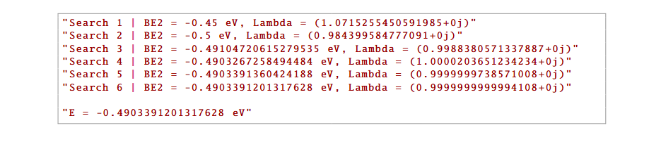
(1) Energy Search / Binding Energy During the iterative solution of the LS equation, you will see a short search log. A typical printout for exciton:
Visual cue: If convergence is slow, lower \(Np\) and \(Nphi\) and then run the cell again.
(2) Hamiltonian Expectation Value Check (only for exciton) Each calculated binding energy \(E\)is checked against the expectation value \(\langle H\rangle = \langle H_0\rangle + \langle V\rangle\) computed from the corresponding wave function. A typical printout for exciton:

Expectation: The relative percentage difference should be very small (near machine precision for well converged binding energies), indicating numerical consistency.
(3) Wave-Function PlotsYou will see momentum space wave functions \(\psi^{(n)}_{m}(p)\) for ground and, when present, excited states. A typical output wave function plot for exciton is shown in Fig 4.
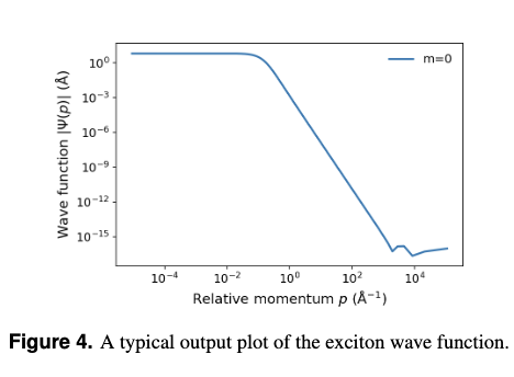
Visual cue: Ground states are typically broader in\(p\); excited states exhibit nodes and shift weight toward lower \(p\) as spatial extent increases.
Saving or Resetting Your Work
Download your edits: Right-click a notebook (i.e. Exciton\(_-\)2D.ipynb) and chooseDownload.
Save figures: Select the plot, then drag and drop it onto your device.
Reset to original: Refresh the page (sessions are ephemeral).
Troubleshooting
Blank or unresponsive: Ensure JavaScript is enabled; refresh the page.
Memory or speed issues: Reduce Np or Nphi; close heavy tabs.
Stuck kernel: Kernel \(\rightarrow\) Restart Kernel.
No changes after edits: Run \(\rightarrow\) Run All Cells.
Quick Checklist
Open a notebook and Run All once.
Edit
Np,Nphi,m, and potential parameters.Restart Kernel and Run All Cells.
Confirm convergence of energy; check \(\langle H\rangle\) vs. \(E\) (small relative percentage difference); inspect wave-function plots.
Download the notebook or images if you wish to keep results.
Cite this work
Please cite the companion article if you use this resource: K. Adderley, K. Mohseni, and M. R. Hadizadeh, “Open-Source Interactive Website for Exciton Modeling via the Lippmann–Schwinger Equation,” https://csu-physics.github.io/2B_2D/ (2025).